Skip to content

MSc-Abschlussarbeit — Universität zu Köln | Betreuer: Prof. Dr. Dominik Wied | 2026

A Test for the Practical Relevance
of Endogeneity in Semiparametric
Distribution Regression

Statistical Theory Semiparametric Econometrics Distribution Regression Instrumental Variables Asymptotic Theory Monte Carlo Simulation R
Forschungsarbeit in Vorbereitung — 2026 Aktueller Entwurf Druckbare Kurzfassung Alle wissenschaftlichen Arbeiten

Worum geht es — und warum ist das relevant?

Problem in einem Satz

Klassische Endogenitätstests sind in großen Stichproben uninformativ — selbst vernachlässigbare Verzerrungen werden mit Wahrscheinlichkeit eins entdeckt und führen zu unnötiger Instrumentalvariablenschätzung, die Präzision kostet ohne inhaltlichen Mehrwert.

Mein Beitrag

Ich entwickle einen Test, der nicht fragt „Ist Endogenität exakt null?", sondern „Verändert die Korrektur die geschätzte bedingte Verteilung um mehr als eine inhaltlich bedeutsame Schwelle Δ?" — eine statistisch wie substanziell fundierte Entscheidungsgrundlage.

Methoden

Semiparametrische Verteilungsregression · Instrumentalvariablen (Control-Function) · Asymptotische Theorie (Einfluss-Funktionen, sequenzielle Linearisierung) · Monte-Carlo-Simulation in R · Empirische Anwendung (Card 1995, n = 3 010)

Ergebnis

Der Test ist asymptotisch pivotal — kein Bootstrap erforderlich. Simulationen bestätigen Niveau α = 0,05 und Konsistenz. Empirisch: Endogenität ist praktisch relevant, aber nur für hochgebildete Arbeitnehmer — ein Befund, den ein klassischer Hausman-Test vollständig verdeckt.

Warum relevant für datengetriebene Entscheidungsunterstützung

Analyseverfahren, die statistische Signifikanz mit praktischer Bedeutsamkeit gleichsetzen, rauschen über das hinaus, was wirklich zählt. Diese Arbeit demonstriert, wie man eine Entscheidungsregel so formuliert, dass sie inhaltlich kalibriert ist — eine Fähigkeit, die überall dort relevant wird, wo Modellaussagen operative oder rechtliche Konsequenzen haben.

Statistische Signifikanz ≠ Praktische Relevanz

Beide Diagramme zeigen dieselbe gemessene Verzerrung d̂ = 0,026. Der Unterschied liegt allein in der Entscheidungsschwelle. (Monte-Carlo-Illustration: n = 1.000, ρ = 0,5.)

Klassischer Hausman-Test

Frage: Ist d > 0?

0 ← Schwelle d̂ = 0,026 0,10
IV erzwungen — d̂ > 0

Jede messbare Abweichung d̂ > 0 führt in großen Stichproben zur Ablehnung — auch wenn die Korrektur inhaltlich bedeutungslos ist.

Praktischer Relevanztest (diese Arbeit)

Frage: Ist d > Δ?

0 d̂ = 0,026 Δ = 0,05 0,10
OLS ausreichend — d̂ < Δ

d̂ = 0,026 liegt unterhalb der Relevanzschwelle Δ = 0,05: Verzerrung statistisch vorhanden, aber inhaltlich bedeutungslos. IV-Schätzung würde Präzision ohne Mehrwert kosten.

Für technische Leserinnen und Leser: vollständige Herleitung

Das Folgende enthält die formale Theorie, Simulationsergebnisse und die empirische Anwendung der Abschlussarbeit. Die Arbeit ist noch in Bearbeitung; theoretisches Rahmenwerk, Asymptotik und Monte-Carlo-Simulation sind abgeschlossen.

Forschungsarbeit in Vorbereitung. Dies ist meine Abschlussarbeit im MSc Volkswirtschaftslehre an der Universität zu Köln, betreut von Prof. Dr. Dominik Wied. Theoretisches Rahmenwerk, asymptotische Beweise und Monte-Carlo-Simulation sind abgeschlossen. Die empirische Anwendung ist als vorläufige Illustration enthalten.

Abstract

We develop a test for the practical relevance of endogeneity in semiparametric distribution regression (DR). Classical tests ask whether the endogenous regressor is exactly exogenous — a question that is uninformative in large samples because even negligible deviations are detected with probability approaching one. We instead test whether correcting for endogeneity changes the estimated conditional distribution by more than an economically meaningful threshold Δ > 0.

The object of interest is the L²-distance d(x,y₂) = ‖F𝑁(·|x,y₂) − F𝑉(·|x,y₂)‖₂ between the ordinary DR estimator and the control-function IV-DR estimator of Wied (2024). The resulting test statistic is asymptotically pivotal: its limiting distribution under the boundary d = Δ is that of a ratio of Brownian-motion functionals, whose quantiles can be obtained by simulation once and for all. The test is consistent and detects local alternatives at rate n⁻½.

L₂-Distance
New functional object: distance between naive and IV-corrected conditional distribution estimates
Pivotal
No bootstrap, no variance estimation — limiting distribution is a Brownian-motion ratio, simulatable once
n⁻½
Consistent test, detects local alternatives at the parametric rate
Card (1995)
Returns-to-education application: endogeneity practically relevant only for high-education workers

1. The Problem with Classical Endogeneity Tests

A central challenge in applied microeconometrics is deciding whether to use instrumental variables (IV) estimation. IV is consistent under endogeneity but less precise than OLS. The conventional approach relies on Hausman-type tests of exact exogeneity: if the null is rejected, switch to IV. This creates a well-known trap.

Classical Hausman Test (Problem)

  • Tests: is endogeneity exactly zero?
  • In large samples, even economically negligible correlations are detected with probability → 1 (Berkson 1938; Hodges & Lehmann 1954)
  • Forces IV estimation even when bias is trivially small — at a precision cost that outweighs the benefit
  • Summarises all evidence in a single mean-based scalar, missing distributional heterogeneity
  • Not designed to answer the practically relevant question

Relevant-Endogeneity Test (This Paper)

  • Tests: does correcting for endogeneity change the conditional distribution by more than Δ?
  • Practically motivated threshold Δ is set by the researcher on substantive grounds before seeing the data
  • Profile-specific: can identify that endogeneity matters for some subgroups but not others
  • Operates on the entire conditional distribution — captures heterogeneous distributional effects
  • Directly answers whether IV correction is worth its precision cost
"The appropriate question is not whether endogeneity is exactly zero but whether it is large enough to matter practically." — Paper, Introduction

This perspective belongs to the equivalence-testing and minimum-detectable-effect literatures (Wellek 2010; Lakens 2017), but has received little attention in distributional models. This paper fills that gap for semiparametric distribution regression.

2. Distribution Regression and the Structural Model

Distribution Regression

Distribution regression (DR), introduced by Foresi & Peracchi (1995) and developed by Chernozhukov, Fernández-Val & Melly (2013), models the entire conditional distribution function of an outcome Y given covariates X:

DR Model FY|X(y|x) = Λ(x'β(y))

where Λ is a known link function (e.g. probit or logit) and β(y) varies with the threshold y. Each y-binary regression 1{Yₐ ≤ y} = Λ(Xₐ'β(y)) + Uₐ(y) is estimated separately, yielding a flexible nonparametric description of the full conditional distribution. Unlike quantile regression, DR handles mass points and non-smooth distributions naturally, and avoids bandwidth choices.

Structural Model with Endogeneity

When the regressor Y₂ is endogenous — correlated with the latent error U(y) — the standard DR estimator is inconsistent for the structural conditional distribution. The paper adopts a triangular simultaneous-equations structure:

Structural Equations 1*y = X'β1(y) + Y2β2(y) + U(y)
Y2 = X'γ1 + Z'γ2 + V

Endogeneity enters through the error decomposition U(y) = α1(y)V + α2(y)ε(y), where α1(y) ≠ 0 induces correlation between the structural error and the first-stage residual V. Using instruments Z and the control-function approach of Rivers & Vuong (1988), Wied (2024) proposes a three-step IV-DR estimator that recovers the structural distribution.

Three-Step IV-DR Estimation

1

First Stage (OLS)

Regress Y₂ₐ on (Xₐ, Zₐ) by OLS to obtain estimated first-stage residuals V̂ₐ = Y₂ₐ − Aₐ'Γ̂.

2

Control-Function Binary Choice (MLE)

For each threshold y, estimate the augmented binary choice model that includes V̂ₐ as an additional regressor, treating it as the control function.

3

Average over Residual Distribution

Integrate out unobserved heterogeneity V by averaging over the empirical distribution of V̂ₐ, obtaining the average structural distribution F𝑉(y|x,y₂).

3. The Relevant-Endogeneity Test

The Endogeneity Distance Functional

The practical endogeneity distance at covariate profile (x,y₂) is the L²-norm of the pointwise difference between the naive and IV-corrected conditional distribution functions over the outcome interval I:

Practical Endogeneity Distance d(x,y₂) = ‖δ(·|x,y₂)‖2,I = (∫I δ(y|x,y₂)² dy)1/2

where δ(y|x,y₂) = F𝑁(y|x,y₂) − F𝑉(y|x,y₂)

Hypotheses

Relevant-Endogeneity Hypotheses H₀: d(x,y₂) ≤ Δ     (endogeneity is practically irrelevant)
H₁: d(x,y₂) > Δ     (endogeneity is practically relevant)

Rejecting H₀ means that correcting for endogeneity changes the estimated conditional distribution by more than Δ over I. Failing to reject means endogeneity is practically irrelevant at that covariate profile, regardless of statistical significance.

Threshold Calibration

The threshold Δ must be chosen before observing the data on substantive grounds. Two natural approaches:

Benchmark Shift
Δ²c = ∫I [FY(y) − FY(y−c)]² dy — calibrated to the L²-distance of a meaningful c-unit shift in the outcome distribution
Fraction of Variance
Δ² = η · ∫I FY(y)(1−FY(y)) dy — normalizes the threshold as a fraction η of marginal variance

Test Statistic and Decision Rule

The test statistic is the full-sample integrated squared distance:

Test Statistic & Decision Rulen(x,y₂) = ∫I δ̂(1,y|x,y₂)² dy

Reject H₀ at level α if: n(x,y₂) > Δ² + q1−αn(x,y₂)

The self-normalizing term V̂n(x,y₂) is constructed from sequential (partial-sample) versions of both estimators, adapting the self-normalization device of Dette, Möllenhoff & Wied (2025) to the one-sample correlated setting. The quantile q1−α is that of a Brownian-motion ratio W = B(1) / (∫ε1(B(t)/t − B(1))² dt)1/2 — simulatable to arbitrary precision with q0.95 ≈ 1.755 for ε = 0.1.
4. Asymptotic Theory

The theoretical contribution requires combining three distinct bodies of asymptotic theory, because the naive and IV-DR estimators are estimated from the same data — creating a non-trivial correlation structure absent in the independent two-sample case.

Joint Influence-Function Representation

Derives the influence functions φNi(y) and φVi(y) for the naive and IV-DR estimators jointly, accounting for their dependence. The IV influence function requires four steps: first-stage OLS expansion, generated-residual Taylor expansion, Z-estimator expansion for the control-function MLE, and the final averaging step.

Sequential Asymptotic Linearity

States a high-level sequential (partial-sample) linearization condition under which √n{δ̂(t,y) − δ(y)} = (√n/nt) Σi=1nt ξi(y) + op(1) uniformly in (t,y) ∈ [ε,1]×I. Primitive sufficient conditions given in Proposition 5.1.

Pivotal Limit via Self-Normalization

The key observation is that both √n(T̂n−T) and √n V̂n converge to τ times a Brownian-motion functional. The τ cancels in the ratio (T̂n−T)/V̂n, giving the pivotal limit W — free of nuisance parameters without bootstrap.

Main Theorem (5.7)

Under Assumptions 5.1–5.5, the test has asymptotic level α on the null d ≤ Δ, exact asymptotic level α on the boundary d = Δ, is consistent against d > Δ, and detects local alternatives at rate n−1/2 (Corollary 5.8).

"No bootstrap and no variance estimation are required. The test statistic is asymptotically pivotal under d = Δ — a ratio of Brownian-motion functionals whose quantiles can be simulated once and for all."

5. Monte Carlo Evidence

Simulations use a triangular model with one exogenous regressor X, one instrument Z, one endogenous regressor Y₂, and a continuous outcome Y. The endogeneity strength is controlled by ρ ∈ [0,1) — when ρ = 0, Y₂ is exogenous; when ρ > 0, Y₂ is endogenous. Distribution regression is implemented using a probit link, evaluated at the covariate profile (x, y₂) = (0, 0). Sample size n = 1,000; nominal level α = 0.05.

Interior Null: Endogeneity is Present but Not Practically Relevant (Δ = 0.05)

Table 1 shows that even at ρ = 0.5 — substantial correlation between structural error and first-stage residual — the estimated distance d̂ = 0.026 remains below the relevance threshold Δ = 0.05, and the test correctly does not reject.

ρΔnRejection rateMean T̂nMean d̂
0.00.0510000.002.82 × 10−⁶0.0014
0.20.0510000.003.95 × 10−⁶0.0057
0.50.0510000.007.23 × 10−⁴0.0263
B = 100 Monte Carlo replications. The test does not reject when d < Δ, regardless of statistical significance of endogeneity.

Power as the Relevance Threshold Varies (ρ = 0.5)

Table 2 shows power as Δ varies. Rejection probability decreases as Δ increases — the test is sensitive to the threshold rather than merely to the presence of nonzero endogeneity. The transition occurs near Δ ≈ 0.027, consistent with the estimated distance d̂ ≈ 0.027.

ρΔnRejection rateMean d̂
0.50.00510000.650.0284
0.50.01010000.620.0268
0.50.02010000.210.0274
0.50.03010000.010.0269
0.50.04010000.000.0279
0.50.05010000.000.0277
Power decreases monotonically with Δ. Transition near Δ ≈ 0.027 confirms the test targets practical relevance, not mere statistical significance.

Boundary Behavior (ρ = 0.5, Δ = 0.027)

When Δ is set close to the true distance d(x,y₂) ≈ 0.027, rejection rates converge to the nominal level α = 0.05 for both n = 1,000 and n = 2,000, confirming the theoretical prediction of Theorem 5.7.

6. Empirical Application: Returns to Education

The test is applied to Card's (1995) returns-to-schooling data (n = 3,010), where education is treated as potentially endogenous and proximity to a four-year college (nearc4) serves as the excluded instrument. Controls include experience, experience squared, Black, SMSA, and South indicators.

Benchmark: Mean-Based Analysis Finds No Evidence of Endogeneity

The standard linear Wu–Hausman test fails to reject exogeneity (p-value = 0.215), despite the OLS estimate (0.0740) and the IV estimate (0.1323) differing substantially in magnitude. This motivates asking a distributional question: even if mean endogeneity is not statistically detectable, does the IV correction shift the distribution of log wages by a practically relevant amount?

Profile-Specific Relevant-Endogeneity Test

The test is applied at three covariate profiles representing low (educ=10, exper=4), middle (educ=13, exper=8), and high (educ=17, exper=15) education/experience workers. The findings are strikingly heterogeneous.

ProfileΔnCritical valueReject?
Low
(educ=10)
0.010.02190.14790.0254No
0.020.02190.14790.0257No
0.030.02190.14790.0262No
0.050.02190.14790.0278No
Middle
(educ=13)
0.010.00090.03040.0129No
0.020.00090.03040.0132No
0.030.00090.03040.0137No
0.050.00090.03040.0153No
High
(educ=17)
0.010.03800.19490.0353Yes
0.020.03800.19490.0356Yes
0.030.03800.19490.0361Yes
0.050.03800.19490.0377Yes
Baseline specification. ε = 0.2, central 10–90% log-wage grid with 31 points, q0.95 ≈ 2.69. Rejection rule: T̂n > Δ² + q1−αn.
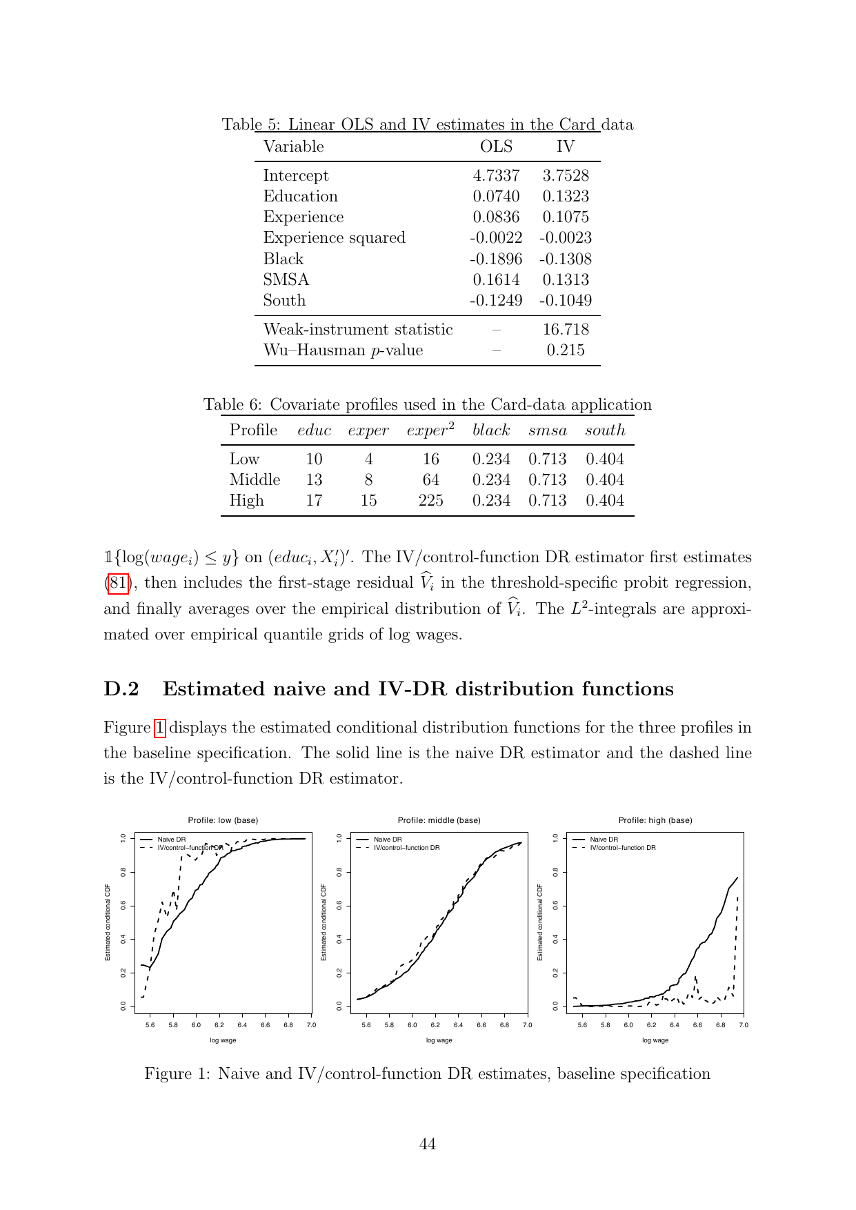
Endogeneity is Practically Relevant — But Only for High-Education Workers The scalar Wu–Hausman test misses this heterogeneity entirely. Distribution regression reveals that the IV correction changes the conditional wage distribution by a practically meaningful amount (d̂ = 0.195) for high-education workers, while the middle profile shows only small differences (d̂ = 0.030). This is a distributional finding, not a mean-based one.

Estimated Conditional Distribution Functions

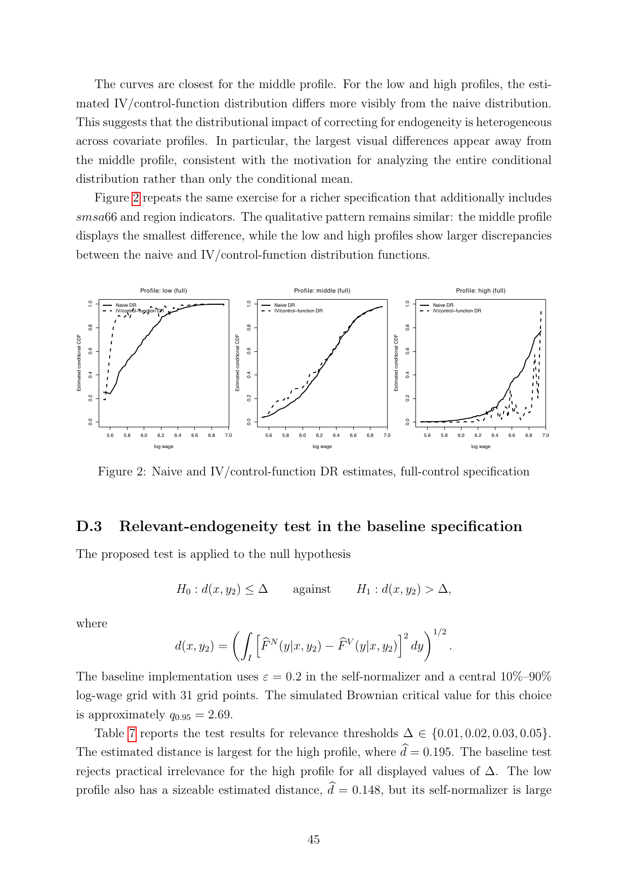
Figures 1 and 2 plot the estimated conditional CDFs of log wages for naive DR (solid) and IV/control-function DR (dashed) at the three covariate profiles. The curves are closest for the middle profile; the low and high profiles show visibly larger discrepancies — especially the high profile, where the IV correction shifts the distribution substantially.

Figure 1
Naive and IV-DR Estimates — Baseline Specification
Naive DR and IV control-function DR conditional CDF estimates for three covariate profiles, baseline specification

Baseline controls (experience, experience², Black, SMSA, South). Solid: naive DR; dashed: IV-DR. The high-education profile (right panel) shows the largest gap.

Figure 2
Naive and IV-DR Estimates — Full Specification
Naive DR and IV control-function DR conditional CDF estimates, full control specification

Full controls (baseline + smsa66 + region indicators). Qualitative pattern persists: middle profile closest, low and high profiles most discrepant. Formal rejection for the high profile disappears with the richer control set.

7. Extensions

Aggregated Version

Integrates the pointwise test over all covariate profiles with weight measure μ, yielding a global relevance test D² = ∫ ∫ [F𝑁(y|x,y₂) − F𝑉(y|x,y₂)]² dy dμ(x,y₂). Natural choices: empirical, policy-relevant, or population measure.

Monotonicity Correction

DR estimators are not guaranteed monotone in y in finite samples. Both monotone rearrangement (Chernozhukov et al. 2010) and isotonic regression (Wied 2024) can be applied — the √n-convergence rate and Gaussian limit carry over.

Confidence Sets for d(x,y₂)

Inverting the test gives a one-sided lower confidence set [Δ̂α, ∞) for the practical endogeneity distance, providing a data-driven summary of endogeneity magnitude at each covariate profile.

Multiple Endogenous Regressors

The framework extends to Y₂ ∈ ℝm with m > 1 endogenous regressors and ℓ ≥ m instruments. The first stage becomes a system of linear equations; the asymptotic results carry over under multivariate generalizations.

Key Literature

Wied (2024)
Semiparametric distribution regression with instruments and monotonicity. Labour Economics, 90:102565.
Dette, Möllenhoff & Wied (2025)
Practically significant differences between conditional distribution functions. arXiv:2506.06545.
Chernozhukov, Fernández-Val & Melly (2013)
Inference on counterfactual distributions. Econometrica, 81(6):2205–2268.
Rivers & Vuong (1988)
Limited information estimators and exogeneity tests for simultaneous probit models. Journal of Econometrics, 39(3):347–366.
Card (1995)
Using geographic variation in college proximity to estimate the return to schooling. Essays in Honour of John Vanderkamp, pp. 201–222.
van der Vaart & Wellner (1996)
Weak Convergence and Empirical Processes. Springer. [Theoretical foundation for functional CLTs and Z-estimators in function spaces]
Hodges & Lehmann (1954)
Testing the approximate validity of statistical hypotheses. J. Roy. Stat. Soc. B, 16(2):261–268. [Motivates the practical-relevance framing]
Foresi & Peracchi (1995)
The conditional distribution of excess returns. JASA, 90(430):451–466. [Original distribution regression paper]
Alle wissenschaftlichen Arbeiten Druckbare Kurzfassung Aktuellen Entwurf herunterladen